Recurrent Neural Networks (RNNs) - Intuition, Math, and BPTT

So this is going to be a comprehensive blog on Recurrent Neural Networks (RNNs) - so far we have learnt about FCNNs, CNNs, etc. But they all have something missing, something which the human brain specialises in. Can you guess it?

Ok let me spill it, it's memory!

Why RNNs?

So before we move onto the concept of RNNs, let's discuss why it came into discussion in the first place. Regular neural networks, be it FCNNs, CNNs, etc. all work the same way:

input → hidden layers → output

Once the output is produced, the network forgets everything.

The next input you pass in the next time step has no relation to the previous one. The model is stateless.

Think of it like HTTP: each request is independent, no memory of past requests.

To be concise: vanilla neural networks do not have memory. It cannot refer to what the past input was and it cannot relate the present input with the past inputs, this limits the Neural Network from identifying trends, patterns, etc. And if you just look back, RNNs are one of the most fundamental concepts which lead to the current day technology in AI by unlocking the capability of NN's to have memory.

So Why Do We Need Memory?

Let's take a classic NLP example:

"My dog has blue eyes, it loves its new pet toy that I bought."

When the model encounters the word "it", what does it refer to?

• the dog?
• the eyes?
• the toy?

A standard neural network has no idea, because it processes inputs independently.

This is exactly the class of problems where context matters. Language, time series, speech, sensor data, sequences in general have a certain pattern/trend and we need memory to predict the next term in the sequence( The sequence could be language, audio, etc.)

RNNs for the Rescue

Instead of treating each input independently, an RNN processes inputs sequentially. Now what does this mean?

An RNN is made up of recurrent cells. At every time step $t$, the cell takes two inputs:

1. the current input $x_t$
2. the previous hidden state $h_{t-1}$

It then produces:

• a new hidden state $h_t$
• optionally an output $y_t$

Now this is where RNNs are different from regular NN's, instead of the output from one hidden layer passing through the next hidden layer, here in RNNs the hidden state produced in the first time step passes through the same Recurrent Cell in the next time step. Notice that the weights are shared here for all the time steps. We see something similar in CNNs where the kernel values are shared, and we know why sharing weights are such a huge improvement, both in learning the features and reducing the number of computations

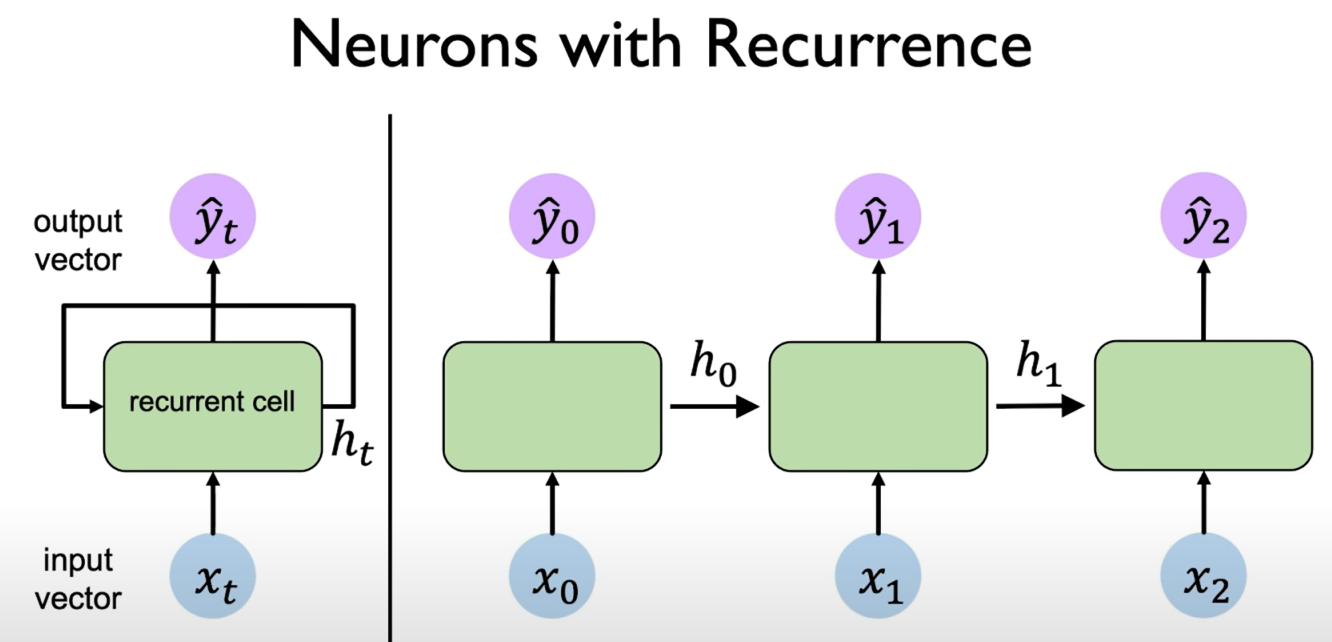
Image credit: authurwhywait.github.io

Now What Is the Hidden State?

The hidden state is the memory of the network.

Think of it as:

"everything the network has understood so far compressed in a vector numerically"

Let's say you(RNN) are a student studying history, now here is how an RNN works:

• You initialise an empty Hidden state vector
• You take in the first embedding of the word from your textbook as the input at time step 0, now you encode this information into the hidden state
• Now you take in the next word at time step 1, now you use the knowledge you learnt from the previous word to process the input and then write the new encoded knowledge to the hidden state
• This goes on and on
• At any time step you can make a prediction y, from the current hidden state

The Core RNN Equations

Hidden state update:

Output:

Where:

• $W_{hh}$ → recurrent (memory) weights
• $W_{xh}$ → input weights
• $W_{hy}$ → output weights

A Key Property: Weight Sharing

The same weights are used at every time step.

This is what allows RNNs to generalize across sequences of different lengths.

Backpropagation Through Time (BPTT)

Here in RNNs we use some thing known as Backpropagation Through Time, now as the name suggests, we travel back through the time steps to reduce the loss. BPTT is just backpropagation with a twist.

Instead of going backward through layers, we go backward through time.

The Big Picture

An RNN unrolled through time looks like a very deep network:

x₁ → h₁ → h₂ → h₃ → ... → h_T

Each hidden state depends on the previous one. So when we compute gradients, the error must flow backward across time steps.

The Core Gradient Equation

The heart of BPTT is this( It's a wonderful derivation, hope you work it out on paper ):

This single equation explains everything.

Intuition: Two Sources of Blame

The hidden state $h_t$ is blamed in two ways:

1. Local Error (Present)

If the prediction at time t is wrong:

This is the immediate mistake.

2. Future Error (Butterfly Effect)

$h_t$ also influences all future hidden states. So if something goes wrong later, $h_t$ is partially responsible.

That error flows back through:

The tanh "Valve"

The derivative of tanh is:

This acts like a valve:

• if neuron is active → gradient flows
• if neuron is saturated → gradient dies

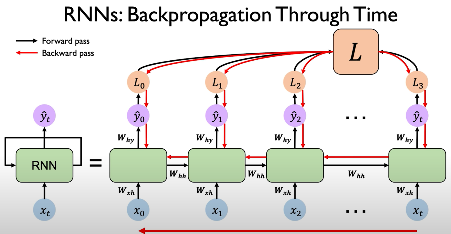
Image credit: authurwhywait.github.io

Why Gradients Vanish in RNNs

Now let's address the main issue in RNNs, which is vanishing gradients. We all know that the range of tanh(z) is [-1, 1]. So the derivative as we saw aboove should always be <=1. So Each timestep multiplies the gradient by a value less than 1.

After $T$ steps( if we take 0.5 as the average value ):

For large $T$, this becomes almost zero.

If we just look back to the loss equation, after many timesteps, the gradient simply does not flow from the future because the tanh derivative part becomes very close to 0 and the weights stop updating, or in other words the network stops learning

That's why: Vanilla RNNs only remember short-term dependencies

Let's discuss the Limitations of Vanilla RNNs

• Vanishing gradients
• Poor long-term memory
• Training becomes unstable for long sequences
• Difficult to capture long-range dependencies in language

All these things led to a newer architecture using the base concept of RNNs, called LSTMs which we will learn about in the next blog.

I hope this blog gave you a baseline intuition on RNNs

Signing off, Gagan